All projects
BACHELOR THESIS / 2024

Turning focus
into depth.

I built and characterized an optical measurement system that turns a sequence of differently focused images (focal stack) into a 3D depth map. The work connects experimental setup design, two configurable MATLAB pipelines and validation against physical reference measurements.

Optical metrologyComputer visionMATLABSolidWorks
SEM focal stack of tin spheres on a carbon substrate.
2MATLAB reconstruction pipelines
3imaging systems applied
10measurements per validation series
01 / THE METHOD

Where an image is sharpest tells us its depth.

A focus measure operator quantifies the sharpness of a local image region. Its values across the known focus positions form a focus function. The position of the fitted maximum gives an estimated surface height. Repeating this across the image produces a depth map.

  1. 01

    Focal stack

    Record the same surface at a sequence of known focus positions.

  2. 02

    Evaluation window

    Follow a small window through every image in the stack.

  3. 03

    Focus function

    Apply a focus measure operator and plot local sharpness against focus position.

  4. 04

    Fitted maximum

    Fit a curve and use the position of its maximum to estimate depth.

  5. 05

    Depth map

    Repeat across the image to reconstruct the surface height.

PROGRAM 1 / DETAILED RECONSTRUCTION

Overlapping evaluation windows, one depth estimate per pixel.

Program 1 moves the evaluation window shown in the workflow across the image one pixel at a time. At each position, the same region is evaluated throughout the focal stack to estimate depth. These overlapping evaluation windows produce a dense depth map and allow spatial smoothing through the window size, at the cost of more computation.
PROGRAM 2 / FAST PARAMETER EVALUATION

Non-overlapping windows, faster feedback.

Each image block produces one depth estimate. This reduces computation and makes it easier to compare processing settings before using them in the denser pipeline. Larger blocks reduce noise while coarsening the output grid.

I compared seven focus measure operators, including GLVA, GLLV and Helmli, and made the window size, curve-fitting method and filtering configurable. The most useful configuration depends on the sample’s texture, illumination and imaging system.

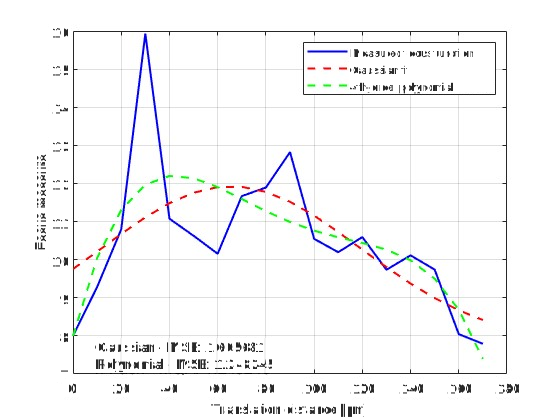
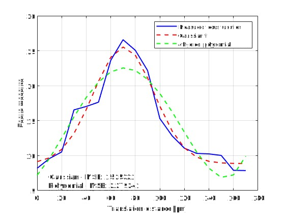
Focus functions: how window size affects the depth estimate

These examples evaluate the same image position with different window sizes. A larger window averages over more structure, changing the focus function and the location of its fitted maximum. Gaussian and fourth-order polynomial fits can therefore lead to different depth estimates.

Focus function for a 64 by 64 pixel evaluation window, with measured sharpness values and Gaussian and fourth-order polynomial fits
64 × 64 px window. The sampled focus function has several local peaks.
Focus function for a 128 by 128 pixel window at the same location, showing a more pronounced peak and the two curve fits
128 × 128 px window. In this example, the main peak is easier to distinguish.
02 / FOCUS IN MOTION

The images behind the reconstruction.

The movies show the plane of focus moving through each scene. The limited depth of field causes local sharpness to change with focus position, providing the physical depth cue used in Shape-from-Focus.

OPTICAL MICROSCOPY

Drosophila compound eye

Watch the eye facets and fine hairs come into focus at different depths. The focus measure operator detects these local changes in sharpness.

92 focus planes · 5 µm axial sampling
SCANNING ELECTRON MICROSCOPY

The same focus planes, before and after registration.

In the original stack, the image shifts laterally as focus changes. A fixed evaluation window then samples different structures, distorting the focus function. Registration aligns corresponding features before depth reconstruction.

Before: unregisteredThe sample moves across the image as focus changes.
After: registeredSURF feature detection and matching keep corresponding structures aligned.

28 matching planes from the original 30-plane stack, shown at the same focus positions. Black margins in the registered images come from shifting the frames.

See the effect on the reconstructed depth maps
03 / MEASUREMENT SETUP

Build the system. Characterize the optics.

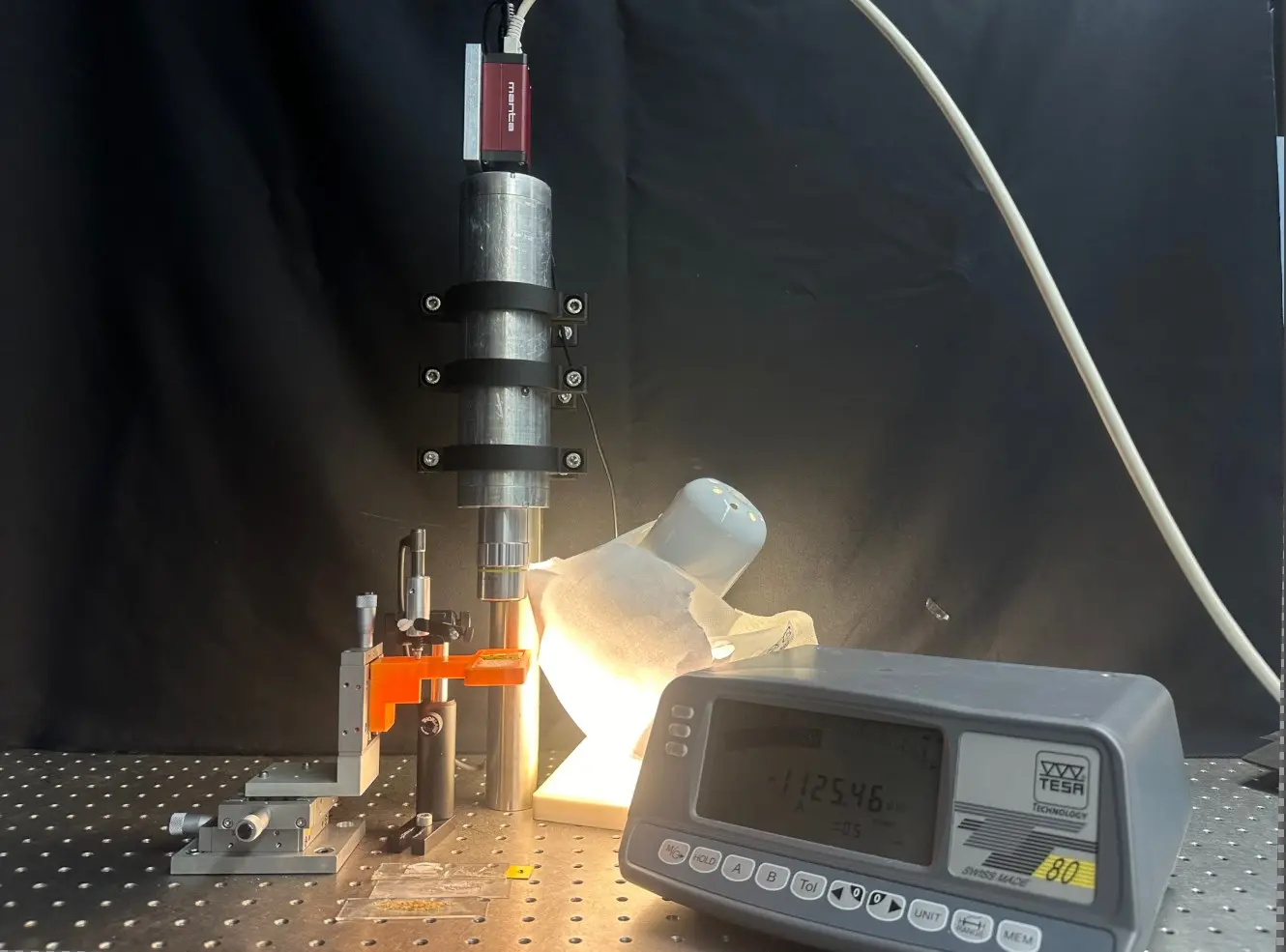
I assembled a compact microscope-based setup, designed and 3D-printed the sample holder and clamps, and added a displacement gauge to measure the sample’s axial position more precisely. Image scale, edge response and depth of field were characterized before evaluating reconstructed heights.

Camera and microscope objective above a sample stage, with illumination and a digital displacement gauge
Experimental setup with imaging optics, a three-axis sample stage, illumination and displacement readout.
ImagingAllied Vision Mako G-319 camera and M Plan Apo microscope objectives; optical characterization with the 20× objective.
PositioningMicrometer translation stages, extended with a Tesa TT-80 readout and displacement probe.
Mechanical designSolidWorks-designed clamps and a 3D-printed slide holder, allowing illumination from above or below.
Image scale
6.88 px/µm
Measured using a stage micrometer; approximately 300 × 224 µm field of view.
Lateral resolution
3.63 µm
10–90% transition width from a knife-edge measurement.
Estimated depth of field
≈ 5.7 µm
Full visually assessed sharp range on an edge tilted by 11°.

These values describe the imaging setup; the reconstruction is evaluated separately below.

04 / VALIDATION

How closely does the reconstructed height match a reference?

I measured the height difference between the surfaces of two razor blades at the blade edge and compared two positioning methods and three curve fits. Each measurement series contained ten focus sweeps. A caliper measurement of six stacked blades gave a 100 µm reference thickness per blade.

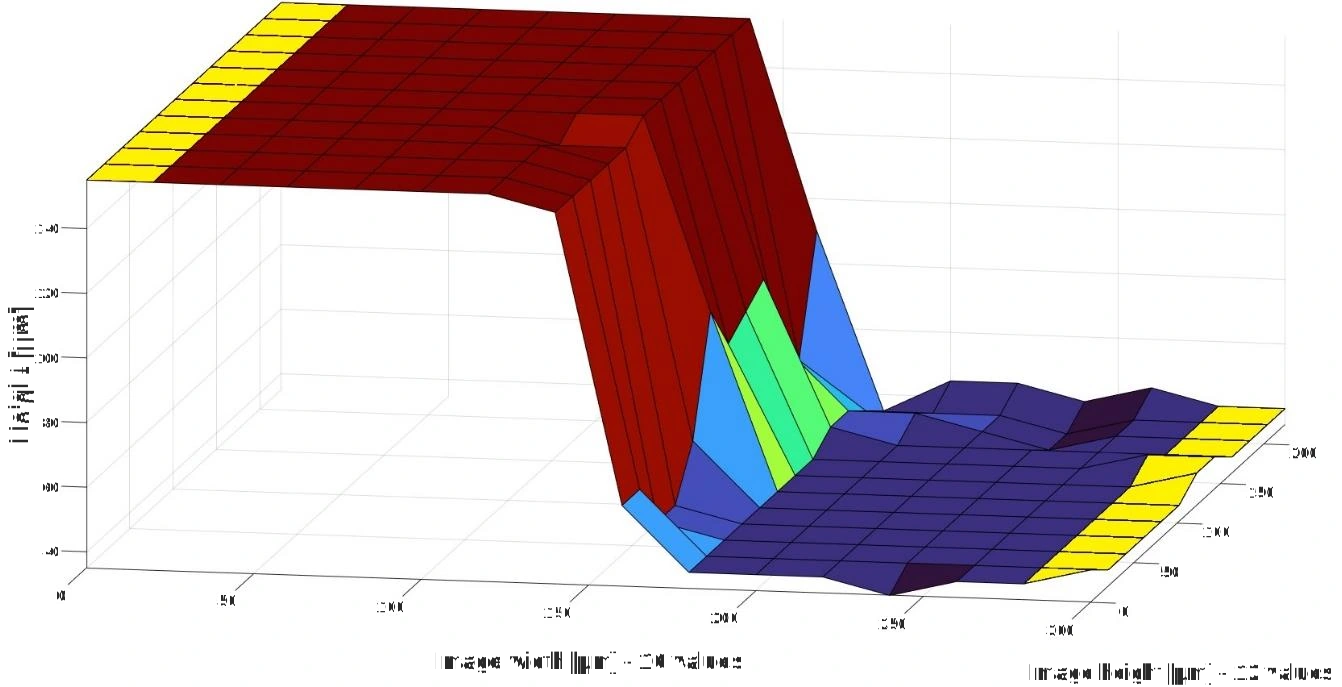
Reconstructed razor-blade step with two plateaus; yellow regions mark the depth samples used to determine the height difference
From a surface to a measurement. The height difference is calculated from the two plateau regions marked in yellow.Program 2 · GLLV · 128 × 128 px windows · fourth-order polynomial · 5 µm translation step.
SMALLEST DEVIATION FROM THE REFERENCE99.00 µm

Mean reconstructed height difference with displacement-gauge positioning and a fourth-order polynomial fit.

Reference thickness
100 µm
Deviation
1%
Standard uncertainty of the mean
1.52 µm
Measurements
10

This result belongs to this sample and measurement configuration. It is not a general 1% accuracy specification for every reconstruction.

Repeatability and deviation from the reference.

With displacement-gauge positioning, the fourth-order polynomial fit yielded a mean height difference of 99.00 µm, closest to the 100 µm reference. The Gaussian fit had the smallest spread, with a standard deviation of 2.68 µm, but its mean was 91.00 µm. The comparison shows that greater repeatability does not necessarily mean a smaller deviation from the reference.

Comparison of six reported means: the displacement-gauge fourth-order polynomial fit gives 99 µm, nearest the 100 µm reference; Gaussian fits give about 89 to 91 µm and second-order polynomial fits overestimate the height difference
Points show means; error bars show the reported standard uncertainty of each mean, based on ten measurements. The dashed line marks the 100 µm reference.
Measurement values and uncertainty notes
Mean ± standard uncertainty, in µm; n = 10 for each series.
Curve fitMicrometer scaleDisplacement gauge
2nd-order polynomial118.17 ± 3.28121.75 ± 1.22
4th-order polynomial90.38 ± 3.3699.00 ± 1.52
Gaussian88.96 ± 2.4491.00 ± 0.85

All six series used Program 2, GLLV and 128 × 128 px windows. For the displacement-gauge series, the standard deviations were 3.84 µm (second-order), 4.81 µm (fourth-order) and 2.68 µm (Gaussian).

05 / APPLICATIONS

One method, three imaging systems.

The MATLAB programs were evaluated across three imaging systems: optical microscopy, scanning electron microscopy and a DSLR setup. Quantitative reference measurements with the microscope were complemented by visual checks of the fly’s-eye reconstruction, geometric plausibility checks of the SEM results, and approximate dimension comparisons in macro imaging.

A / OPTICAL MICROSCOPY

Resolving the structure of a fly’s eye.

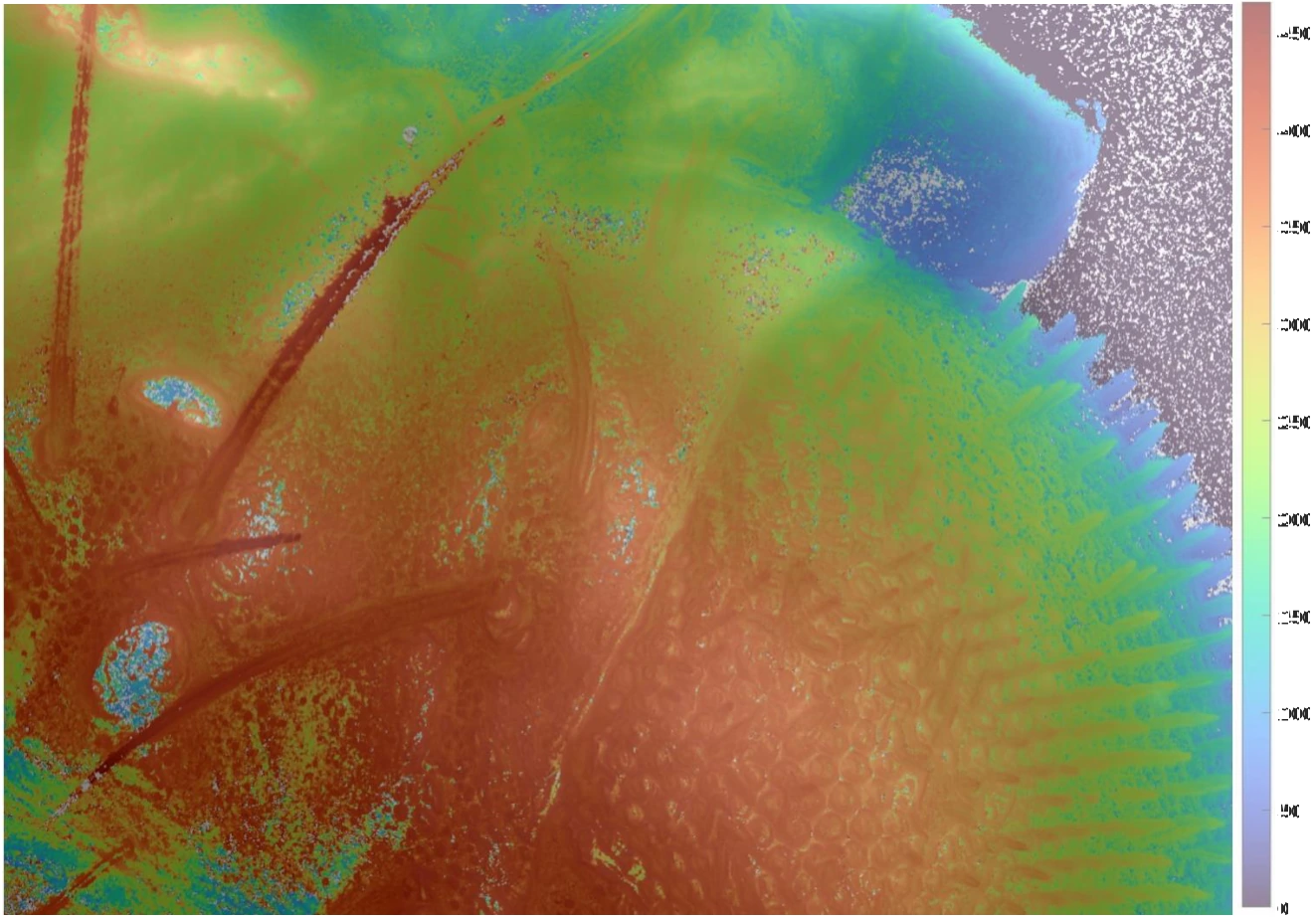
The dense pipeline reconstructs the compound eye and surrounding head. Overlaying the depth map on the image makes it possible to check whether depth changes follow recognizable structures. This is a visual check of the reconstruction.

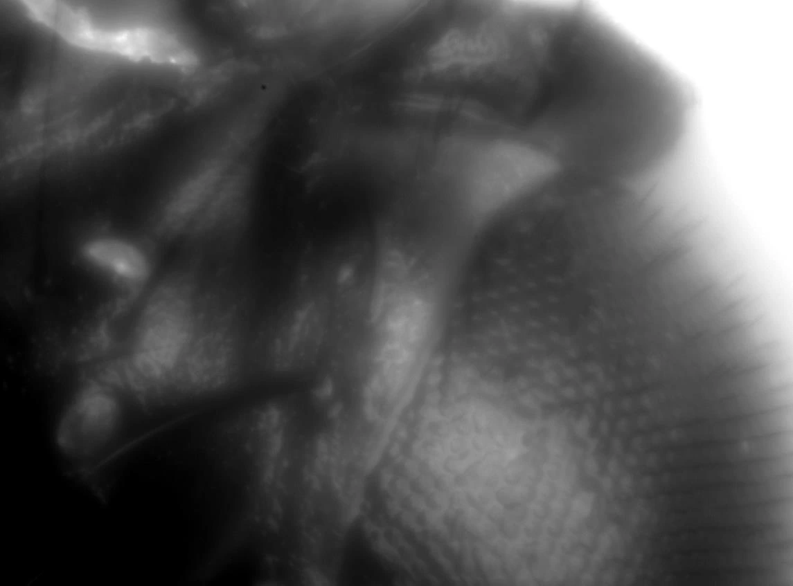
Maximum-intensity projection of a Drosophila head, showing compound-eye facets and hairs
Image reference. Maximum-intensity projection of the focal stack.
Drosophila image with the reconstructed depth map and its micrometre colour scale; eye facets and head contours remain visible
Reconstructed depth overlaid on texture.Program 1 · Helmli focus measure · Gaussian fit · 4 × 4 px windows · 5 µm translation step.
B / ELECTRON MICROSCOPY

Correct image motion before estimating depth.

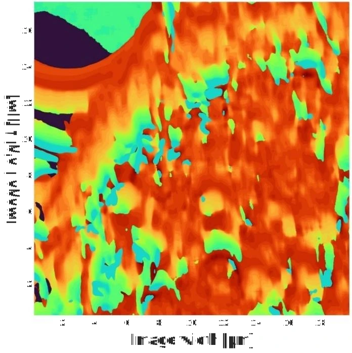
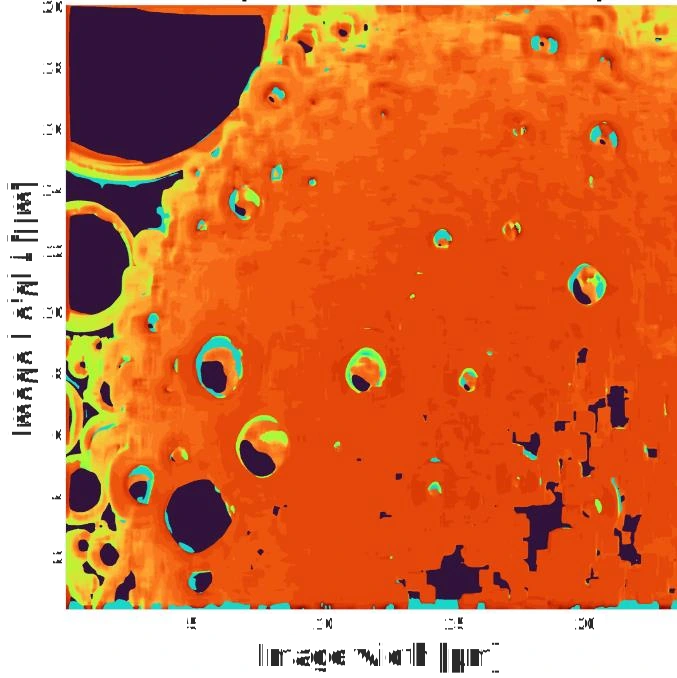
I used SURF feature detection and matching to estimate translations between successive SEM images. Applying cumulative shifts to the original frames keeps the same structures within each evaluation window, so its focus function describes changes in sharpness. The depth maps show how this registration reduces reconstruction artifacts.

Tin-particle depth map before registration, showing distorted surface patterns caused by movement between focal-stack frames
Before registration. Image motion corrupts the local focus curves.
Tin-particle depth map after SURF-based translation alignment, with a more coherent surface shape
After registration. Corresponding structures are evaluated together.

Program 1 · GLVA · fourth-order polynomial · 64 × 64 px windows · 2 µm translation step. Depth plausibility was checked against the SEM scale bar and the approximately spherical geometry; no independent 3D reference scan was used.

C / MACRO IMAGING

Extending the workflow to centimetres.

A Canon EOS 6D setup tested the method on a bowl-shaped object. Changing focus with the lens ring reduced the scale change encountered when moving the camera. A tilted tape measure was used to estimate image scale and focus-position spacing.

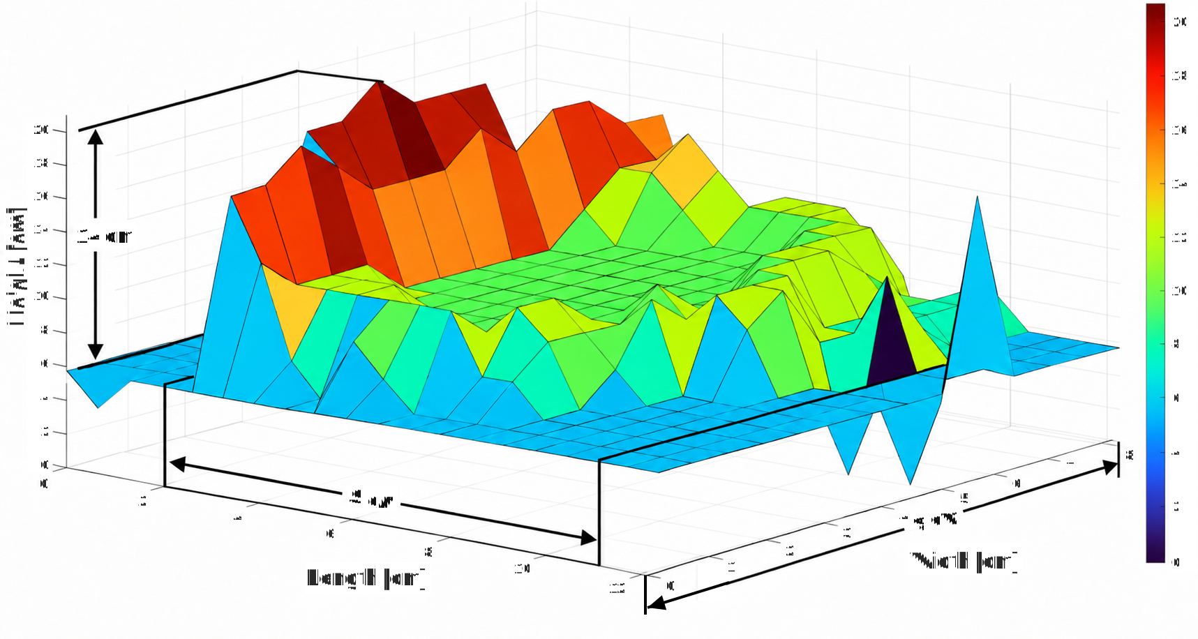
Three-dimensional reconstruction of the bowl-shaped object, with dimension arrows marking a height of 14 cm, a length of 9 cm and a width of 8 cm
Centimetre-scale surface. Program 2 · eighth-order polynomial · 256 × 256 px windows · estimated 1.885 cm focus spacing.
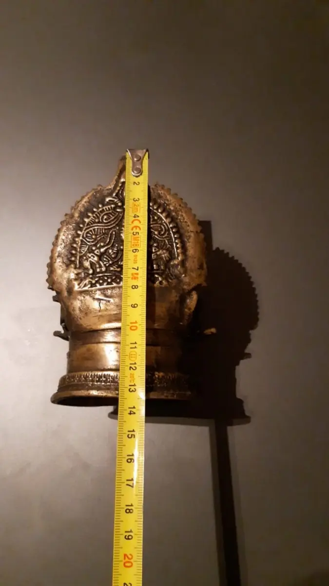
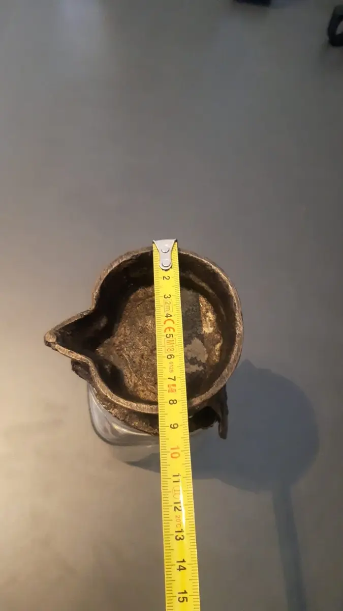
Physical object measured vertically with a tape measure
Reference height measurement.
Width of the bowl measured across its opening with a tape measure
Reference width measurement.
Dimension check against a tape measure.
DimensionReferenceModel
Height13.5 cm14.0 cm
Length9.2 cm9.0 cm
Width8.3 cm8.0 cm

All three checked dimensions differed by less than 5%. This was an approximate dimension check on this object, using estimated image scale and focus-position spacing.

Explore another experiment, measurement system or data workflow.

All selected projects